Lessons in Grafana - Part Three: Mental Metadata

2026-03-09

Welcome back to the main part of the series. Today we will be discussing mental health, and the difficulties of collecting data on it. If you’d rather not read that, then come back next week for a discussion of time tracking.

• 1) A Vision

• 2) Litter Logs

• 2.5) Achieving Acceptable Averages

• 3) Mental Metadata (you are here)

• 4) Noticing Notes

• 5) Graphing Goatcounter

• 6) Bridging Gadgets? Biometrics Galore!

• 7) Plotting Prospective Plans

Prelude and Inspiration

For a long time, I was frustrated whenever I went to my psychiatrist. They would ask me very reasonable questions like “has this medicine improved things?”, and I could not give an answer with certainty. My therapist would point out that I act as if things haven’t gotten better, when from their perspective there had been clear improvements.

This bias was my initial motivation for this project. I wanted to track depression data over time. I wanted to see that things had improved, so I could not ignore that. I wanted to be able to point to a chart and say “yes, doctor, this medication has improved things, you can see here where I started and things got better.” Because I am a person who needs side projects to thrive, it spiraled into all this. I’m pretty happy about that.

Showing progress on this to friends led to them asking how things might be added. Several wanted to use something like this for their own purposes. In the process of listening to that feedback, I added two things that will be featured very prominently in this post: support for tracking anxiety/PTSD symptoms, and support for metadata about Dissociative Identity Disorder and Plurality in general. Because these topics are heavily stigmatized, I once again emphasize: all data in this series is faked and arbitrary. They do not correspond to real people and I will not be identifying anyone who utilizes these features.

Depression Tracking

Depression is famously difficult to quantify [Mit09, PSTF26]. Not only is it an inherently subjective experience, it also is good at disguising itself. To anthropomorphize: depression is a shifty liar. It doesn’t just make you think that things are bad, but that they were always bad and will never get better. Rather than making you feel tired, it can make you feel like you simply have a smaller energy bar in the first place. Measuring something that, by its own nature, tricks you into believing your experience is normal requires questions that reference external factors.

Of course, those are only correlates. You can get better correlations if you ask just the right questions, but there is an amount of error inherent to the fact that you’re measuring the subjective. This has resulted in a vast quantity of questionnaires. You’ll see variations of them at doctors’ offices, on intake forms, or on population surveys.

Because this project was something I had tried before, years ago, I had some idea what I would need to make this work. I was willing to settle for high margin of error, because that’s better than no data at all. The priority for the collection phase was reducing friction at every possible step. The survey should be sent to me without my input. It should require no more than one button press per question. It should minimize the number of questions asked, and allow any with consistent answers to be skipped and inferred.

Because speed of implementation was the biggest priority, I made two immediate decisions:

1. I would design my data collection bot such that it didn’t care what survey I was asking, and

2. I needed to use the shortest survey (after eliminating questions) I could find quickly

What Is The PHQ-9?

The PHQ-9 [Cur] is a self-reported questionnaire consisting of 9 questions. Each of them is assigned a value between 0 and 3, then totaled. The questions are as follows:

Over the last 2 weeks, how often have you been bothered by the following problems?	Not at all	Several Days	More than half the days	Nearly every day
Little interest or pleasure in doing things	0	+1	+2	+3
Feeling down, depressed, or hopeless	0	+1	+2	+3
Trouble falling asleep, staying asleep, or sleeping too much	0	+1	+2	+3
Feeling tired or having little energy	0	+1	+2	+3
Poor appetite or overeating	0	+1	+2	+3
Feeling bad about yourself - or that you’re a failure or have let yourself or your family down	0	+1	+2	+3
Trouble concentrating on things, such as reading the newspaper or watching television	0	+1	+2	+3
Moving or speaking so slowly that other people could have noticed. Or, the opposite - being so fidgety or restless that you have been moving around a lot more than usual	0	+1	+2	+3
Thoughts that you would be better off dead or of hurting yourself in some way	0	+1	+2	+3

This is quite comprehensive, yet can be answered fairly quickly. But 9 questions? Surely we can skip some of these.

Further Compressing

Some of these questions are easy to eliminate. I’ve had sleep inconsistencies my whole life, for example. It just seems to run in the family. That makes it a fairly bad proxy for depression except in the very short term, where there will already be the highest error.

Given that there will be questions like that, let’s write a format that we can store these questionnaires in. We’ll start with the very basics: we want an interval to ask the survey at, and we want a bank of questions.

{
  "randomIntervalHours": [2, 12],
  "questions": []
}

Good! That solves our problem perfectly. Now, what does it look like when we want a question to be asked? Well, one worry that I had from my last attempt at this was about phrasing. If I make it so that the question is identical each time, then that makes your answers habitual. You want to minimize the friction of asking, but if you aren’t careful you’ll find that process automatic. This means not only do we need different phrasings of each question, we also need to shuffle the answers each time we ask. We want you to be forced to actually read the button you’re pushing.

In addition to that, we need to have an indicator that it should be displayed. Otherwise, how do we know when something is to be skipped? And, of course, we need to hold the answer bank. This approach generalizes well.

{
  "question": [
    "In the last two weeks, how often have you had little interest or pleasure in doing things?",
    "In the last two weeks, how often have you lacked motivation or enjoyment in your usual daily tasks?",
    "En las últimas dos semanas, ¿qué tanto has sentido que no quieres hacer nada o que nada te da gusto?"
  ],
  "display": true,
  "answers": {
    "Not at all": 0,
    "Several days": 1,
    "More than half the days": 2,
    "Nearly every day": 3
  }
}

The other path adds a bit more complication. See, we can’t just skip a question. The scoring process for these questionnaires relies on data from them. This means that we need to infer some value for them, and it’s intellectually dishonest to just say “0”. So the way I approach that is with a thing I barely remembered from high school: confidence intervals.

{
  "question": [   // Why bother with extra phrasings if we're skipping it?
    "In the last two weeks, how often have you had trouble falling or staying asleep, or sleeping too much?"
  ],
  "display": false,
  "floor90": 1,   // This says "I'm 90% sure that it'll be 1 or higher"
  "ceil90": 2,    // Similarly, 90% of the time it should be 2 or lower.
  "floor100": 0,  // And you're completely sure that it will be 0 or higher
  "ceil100": 3,
  "answers": {}   // Answers skipped for brevity
}

So, we have a way to write our questions down. We know what questions to ask. Now, given that the answers just magically appear in our hands, how would we interpret them? (Don’t worry, we cover how they get to you later.)

Interpreting Data

I want to be fully upfront about this before we continue: the method I use to compute a final score is arbitrary. There are absolutely different methods I could use. Some of them might even be better, and I would be happy to talk about any suggestions. With that said, let’s go over how we parse through this data.

For each question, we either get an integer (because we got a concrete answer) or a confidence interval (because we need to infer an answer). Each of the integers can be converted into an infinitely narrow confidence interval. This means that what we’ll get is something like:

	Floor		Ceiling
	100%	90%	90%	100%
1	2	2	2	2
2	0	0	2	3
…	…	…	…	…

Being able to represent it as a table is wonderful because it means we can use the same formula for everything. Now that we have this, we need to get a composite score. That’s going to look like making a composite for each row, then adding them up. Since it seems prudent to weight the narrower range higher, I decided on the following:

\[\dfrac{2(X_{F,90\%} + X_{C,90\%}) + X_{F,100\%} + X_{C,100\%}}{6}\]

Because I want this to serve as a historical record, I save every step of this calculation in the database. This way, if my method of inference changes, I can compare it both by the contemporary method and the current method.

Resulting Chart

This is possibly the longest query in this series, not because it’s complicated, but because we are trying to convey a lot of information. It consists of four subqueries. In the first, we are defining our half life as a constant. In the second, we fetch the raw scores for depression values. In the third, we compute the running averages. In the fourth, we gather the thresholds as defined by the questionnaire. Lastly, we gather all of that together.

WITH c AS (SELECT interval '2 days' AS half_life),

raw_depression AS (
  SELECT respondant, "time", final
  FROM lgbot.depression
  WHERE $__timeFilter("time")
),

avg_depression AS (
  SELECT
    respondant || ' R.A.',  -- concatenation
    "time",
    lgbot.ema(
      final::numeric,
      "time",
      c.half_life / ln(2)
    ) OVER (
      PARTITION BY respondant
      ORDER BY "time"
    )
  FROM c, lgbot.depression
  WHERE "time" BETWEEN (timestamptz $__timeFrom() - c.half_life * 8) AND $__timeTo()
),

thresholds AS (
  SELECT x.respondant, t."time", x.final
  FROM (
    VALUES
  --    ('Severe Depression', 20),
      ('Moderately Severe Depression', 15),
      ('Moderate Depression', 10)
  --    ('Minor Depression', 5)
  ) AS x(respondant, final)
  CROSS JOIN (
    VALUES
      (timestamptz $__timeFrom() - interval '1 second'),
      (timestamptz $__timeTo() + interval '1 second')
  ) AS t("time")
)

(
  SELECT * FROM raw_depression
  UNION ALL
  SELECT * FROM avg_depression
  ORDER BY respondant, "time"
)
UNION ALL
SELECT * FROM thresholds

I want to take a moment to review the last two subqueries.

In avg_depression we are gathering averages. The specific method was covered in the bonus entry Achieving Acceptable Averages [ACa], but since that was optional I will summarize. The function lgbot.ema defines an exponential moving average. That means that the farther away a data point is, the less it affects the average value associated with a given measurement. Specifically it does this according to a half life, which we define as a constant. We are applying a less strict time filter to ensure that past values are included in this average. The value chosen here is 8 times the half-life, which means we only exclude values that have a lower weight than \(2^{-8} \approx 0.0039\).

In thresholds we are using a keyword not yet covered in this series: CROSS JOIN. You can think of this like Python’s itertools.product(). In essence, it is a nested for-loop like so:

for name, value in thresholds:
  for ts in times:
    yield (name, value, ts)

All of this yields the following chart. I specify in the axis that higher PHQ9 scores are worse because I was frequently causing confusion when not specified. The instinct of “higher number good” is quite strong.

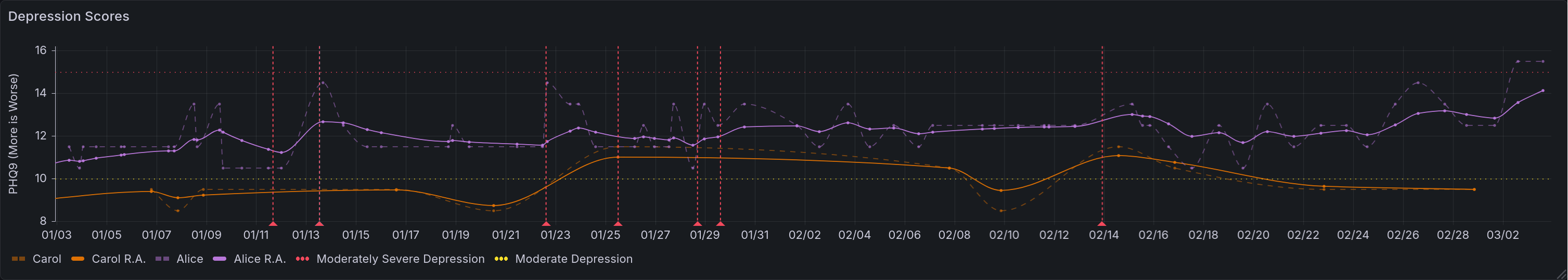
This chart shows depression over time. The Y axis measures the inferred value of the PHQ-9 survey, with higher values being worse. Six lines are shown. Two of them note thresholds for degrees of depression, represented with dotted lines. Two of them note the raw scores for two respondents, represented with dashed lines. The last two show running averages for those respondents, shown in bold. Additionally, there are many dashed vertical lines that are used to denote events related to mental health. Not shown, you can click on them to see details of the events. Many of these correspond to spikes or troughs in raw depression levels.

Survey Delivery and Responses

In Litter Logs [ACc], we showed the overall structure of my tracking bot. Let’s keep building on that, simplifying a bit for clarity.

The biggest new piece here is an integration with Telegram.

Event Loop

The library I use to interact with Telegram is async-by-default, and comes with an event loop. Everything in this bot is driven by that event loop[1]. There are four hooks that enable our data collection:

1. A start() method that sets initial state and handles command callbacks (ex: user sends /phq9)

2. A do_begin_loop() method, instantiated for each survey, which sends the first question once it’s the right time

3. A send_next_question() method that, given a survey, sends the next question in the sequence

4. A questionnaire_callback() method that determines the survey, records the answer, and kicks off either the next question or answer logging

Kicking Things Off

At the beginning of each run, we call start(). It’s fairly straightforward, and looks like so:

async def start(
  update: Update,
  context: ContextTypes.DEFAULT_TYPE,
  bank: BankType
) -> None:
  async with SharedState.lock:
    SharedState.q_asking[bank] = True
    SharedState.q_responses[bank].clear()
    SharedState.q_index[bank] = 0
  await send_next_question(context, bank)

You’ll notice that we are storing three pieces of information. The first piece is just noting that a questionnaire is in progress. This is crucial, because otherwise we might run more than one at the same time. That would be both confusing and annoying. Note that because the start() function is also the command handler, a user can manually trigger multiple questionnaires. If they do so, that’s on them.

The next piece of information is the responses received thus far. This is stored as a list, and is fairly straightforward.

Lastly, we store the index of the last question asked. That might seem strange. After all, we have the list of responses. Why not simply go off of that? Well, because you aren’t getting a response to every question. The index keeps track of where we are in the questionnaire including skipped questions.

Getting Replies

Sending and receiving information through Telegram is relatively easy, but somewhat messy. Because I wanted to minimize friction, we use the on-screen keyboard markup they provide. This means that everything appears as a handy button to click, like so:

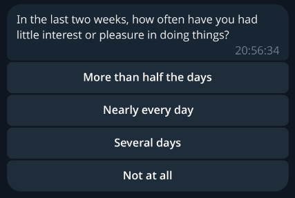
This is an example survey question. In particular, this is the first question of the PHQ-9, as covered above. Note that the answers are scrambled, and appear as a stack of clickable buttons.

In general, we use the following steps:

1. Load information about the next question (covered in the next section)

2. Check if we already asked the final question

3. Construct a keyboard that encodes the questionnaire name and answer label

4. Send the message

5. Receive a reply

6. Decode the questionnaire name and answer label

7. Fetch the answer value

8. Increment question index

9. Delete the message & repeat

This is our message sending method. It handles steps 1-4. The most important thing to pay attention to is the keyboard construction. Note that all of the answers get shuffled using random.sample().

async def send_next_question(
  context: ContextTypes.DEFAULT_TYPE,
  bank: BankType
) -> None:
  """This handles the sending of questions to the user"""
  logger.info("Sending next question for %s", bank)
  (question, answers), num_qs = await gather(
    select_question(bank),
    len_questions(bank)
  )

  async with SharedState.lock:
    if SharedState.q_index[bank] > num_qs:
      ...  # record answers, set up for asking later
      return
    logger.info(
      "%s processing question %i of %i",
      bank,
      SharedState.q_index[bank],
      num_qs
    )

  reply_markup = InlineKeyboardMarkup([
    [InlineKeyboardButton(text=label, callback_data=f'{bank}+{label}')]
    for label in sample((*answers, ), len(answers))
  ])
  await context.bot.send_message(
    chat_id=TELEGRAM_CHAT_ID,
    text=question,
    reply_markup=reply_markup
  )

This is our message receiver method. It handles steps 5-9, and overall has an easier job. The most important thing it does is handling the question index. If it were handled anywhere else, you could have worrying race conditions around what answer gets processed. Handling it here means that, so long as a user does not initiate two of the same survey at once, it will always be processed correctly.

async def questionnaire_callback(
  update: Update,
  context: ContextTypes.DEFAULT_TYPE
) -> None:
  """When answers are submitted, they are processed here"""
  query = update.callback_query
  await query.answer()

  bank, data = cast(Tuple[BankType, str], query.data.split('+'))
  _, answers = await select_question(bank)
  selected = answers[data]
  async with SharedState.lock:
    SharedState.q_responses[bank].append(selected)
    SharedState.q_index[bank] += 1

  await gather(
    query.message.delete(),
    send_next_question(context, bank)
  )

The Annoying Part – Getting Questions

Because we are loading questions dynamically and skipping some of them, deciding which to ask next is somewhat complicated. This is further complicated by needing to preface most questionnaires with information for plural metadata. As a result, this function is pretty messy. It’s definitely not a perfect solution, but is a product of repeatedly making the least modifications possible to accomplish new goals. Rewriting it is one of the things I’d like to do in the near future. With that being said, let’s look at how it works. First I will show code, and then I will attempt to explain the logic in more detail.

# Note: this method may return ('', {}) in an error; detection is on the caller
async def select_question(bank: BankType) -> Tuple[str, Mapping[str, int | str]]:
  question: str = ''
  answers: Mapping[str, int | str] = {}
  async with SharedState.lock:
    if bank == 'poop':  # hack because bodies do what bodies do
      SharedState.q_index[bank] += 1

    if SharedState.q_index[bank] == 0:
      question = f"Who is answering this questionnaire ({bank})?"
      answers = {x: x for x in await load_questions('system')}

    else:
      questions = (await load_questions(bank))['questions']
      try:
        while True:
          index = SharedState.q_index[bank] - 1
          if questions[index].get('display') is False:
            logger.info("%s skipping question %i as requested", bank, SharedState.q_index[bank])
            SharedState.q_index[bank] += 1
          else:
            break
        question = random.choice(questions[index]['question'])
        answers = questions[index]['answers']
      except IndexError:
        pass
  return question, answers

As noted above, this function has many jobs. Arguably it has too many jobs. Its first task is to identify the respondent. Since this bot is designed to have a single user per instance, this is entirely to allow for plural folks to use this better, as covered towards the end of this entry. If this question would ordinarily be asked, we then need to make an exception for things that are pure bodily functions. After all, that is tracking the body not the mind.

Once this task is out of the way, we need to load the main question bank. We start with the first question, checking each time if the question should be skipped. If it should be, then we advance the question index. This is the only other place where that index is advanced. Everywhere else is either reading or clearing it. On the first question that is not marked to skip, we break out of the loop and return. If we do not find such a question, it returns an empty set.

I think that the logic of this is fine, but the implementation details are not my favorite. In my opinion this is the most technically-indebted part of this bot.

Anxiety Tracking

After some time working on this, I was asked why I hadn’t addressed anxiety. After all, that’s something that most people suffer from to some degree, and it can give context to other things. Since psychiatric medicines affect both, it’s rather foolish to measure one without the other.

Anxiety suffers from the same measurement problems as depression, however. On top of that, anxiety has much more moment-to-moment variation. This makes it a lower priority to track, in my opinion, and so I rely on simple self-reporting. The questionnaire for anxiety looks like this:

{
  "randomIntervalHours": [2, 12],
  "questions": [{
    "question": [
      "On a scale of 0 to 5, rate your anxiety",
      "En una escala del 0 al 5, califique su ansiedad."
    ],
    "index": 1,
    "display": true,
    "answers": {
      "0": 0,
      "1": 1,
      "2": 2,
      "3": 3,
      "4": 4,
      "5": 5
    }
  }]
}

Very simple, very pared down. It just asks for a number. And if more precision is ever needed, I can easily migrate it to a more detailed questionnaire. The query used for this is much the same as the one for depression tracking, without the piece about thresholds. For brevity’s sake I will skip it.

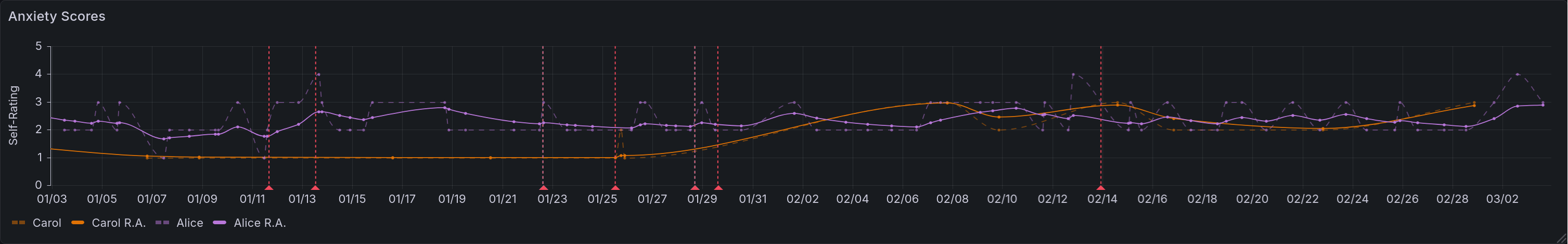
This chart shows anxiety over time. The Y axis measures self-reported anxiety on a scale of 0 to 5, with higher values being worse. Four lines are shown. Two of them note the raw scores for two respondents, represented with dashed lines. The last two show running averages for those respondents, shown in bold. Additionally, there are many dashed vertical lines that are used to denote events related to mental health. Not shown, you can click on them to see details of the events. Many of these correspond to spikes or troughs in raw anxiety levels.

Event Logging

One of the many things this enables is the logging of discrete events. This is anything where the exact timing is unimportant, but knowing that it happened is quite useful.

Toy Example: Poops

The funniest example, and therefore the easiest to talk about, is pooping. Bowel movements. Spending time on the porcelain throne. Not only is this medically useful to track, it also requires the least possible information. With other events, you might need extra information such as duration or severity[2]. So let’s look at how our event handlers treat this.

For one thing, every recorded event is done as a command. In this case, that would be /poop. This calls start(), which calls send_next_question(). This calls select_question() which, as you saw above, is a bit of a mess. Fortunately, it has a short-circuit for this exact use case: we don’t have any questions for this. It just advances the index past the end of the questionnaire, which triggers the end of the survey. Our bot sees we are past the end, and tries to schedule the next one. Let’s look at the file that defines the /poop command:

{
  "randomIntervalHours": null,
  "questions": []
}

Oh my, the random interval is null! This is the nice way to indicate explicitly that we don’t want this to be periodic.

Panic Attacks

Panic attacks require additional information. The biggest of these are the type and the duration.[2]

Because panic attacks often cause a distorted sense of time, the durations we query are intentionally vague. Let’s look at the questionnaire file to see what I mean:

{
  "randomIntervalHours": null,
  "questions": [{
    "question": [
      "How long was this panic attack?"
    ],
    "index": 1,
    "display": true,
    "answers": {
      "For less than 5 minutes": 2.5,
      "For 5-10 minutes": 7.5,
      "For 10-20 minutes": 15,
      "For 20-40 minutes": 30,
      "For 40-80 minutes": 60
    }
  }]
}

By binning the responses like this, we get an idea of severity while minimizing the friction involved in figuring that out. Additionally, we support a second command for this: /flashback. These two are sometimes difficult to distinguish, but the main difference is in emotional context. Panic is about things happening in the present, in the now. A flashback is a memory rearing its head in some way. Sometimes this is as vivid as feeling physically in that moment. Sometimes it is “merely” reliving the emotional context, feeling the internal sensations replayed.

The query for this is incredibly simple:

SELECT
  "time" AS ts,
  respondant,
  "data" AS Panic,
  NULL AS Flashback
FROM lgbot.panic
WHERE $__timeFilter("time")
UNION ALL
SELECT
  "time" AS ts,
  respondant,
  NULL AS Panic,
  "data" AS Flashback
FROM lgbot.flashback
WHERE $__timeFilter("time")

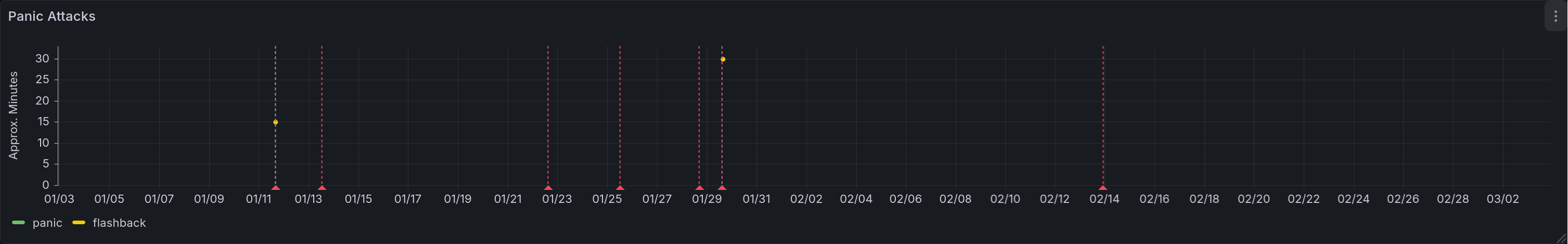
This chart shows panic attacks and flashbacks over time. The Y axis measures rough duration of the events, with higher values being worse. This is rendered as a scatter plot, with a different color representing each type of event. Shown are two panic attacks, with rough durations of 15 and 30 minutes respectively. Additionally, there are many dashed vertical lines that are used to denote events related to mental health. Not shown, you can click on them to see details of the events. Two of these correspond with the panic attacks, providing context.

Plural Metadata

If you aren’t familiar with the topic, you might not know at all what I mean by plurality. There is a lot of nuance here that I am intentionally skipping over, but in general a plural person is someone who experiences multiple identity states[3][4]. These are often called alters[5], facets, or headmates, and this last shall be used throughout this entry. In general there are differences in memory, personality, skill sets, and/or triggers between headmates. Because of that, you can (in general) think of them as having (descriptive) roles for the functioning of the whole. These roles can vary from hyper-specific (they clean our ears) to incredibly general (they handle day-to-day functioning), and some reject the notion of even descriptive roles.

The (set of) headmate(s) that are directly influencing the body are said to be “fronting”. The standard analogy for it is to imagine the body as a car, ship, or plane. You can have a single pilot on some aircraft, but others might need a navigator or an engineer as well. If you’re operating the vehicle, you’re in the front seats, hence fronting.

Knowing that much, you can see why it might be useful to track information about the state of your system, your set of headmates. Having some idea of who is fronting during particular times can be vital to figuring out what works best. This is even more important because systems often suffer from memory issues. In my experience from knowing many, that is particularly true of ordering events.

Who Is Most Helped By This?

I think of plurality as having three axes: population [Sys], partitionality [SSS+], and distinctness [LFfcad7]. This isn’t a universal framework, but it does help explain the target audience for this sort of tracking.

Population

Your system is highly populous if there are more alters/headmates/facets in it. Polyfragmented systems are at the extreme end of this spectrum. Minimal population for the target audience is 2.

Partitionality

Your system is highly partitioned if amnesia barriers between headmates are high. The less able you are to remember what others did while away from front, the more partitioned you are.

Distinctness

Your system is highly distinct if you are able to consistently identify who is at front. Each of you is then clearly distinct internally.

The audience that is most likely to benefit from this kind of tracking are systems that are low in population (of fronters), and high in partitionality and distinctness. If they are high in population, then keeping track of all data points is going to be cumbersome. If they are not very partitioned, then this data is less useful because memory may provide a decent substitute. If they are not very distinct, then determining what to mark in the tracking data is very difficult. While this information is most easily collected for this group, it may still be helpful to others, but on a less consistent basis.

With this target audience in mind, let’s look at what data we can easily gather. All of it can be gathered with a standard time tracker. This specific example is from the Time Slip plugin for Joplin. I’ll provide more detail on data extraction in the next entry, but the format we get is:

Project	Task	Start	End	Duration
text	text	timestamp	timestamp	interval

Current Fronter(s)

The most conceptually simple metric to look at is who is currently fronting. Unfortunately, the query to find this is fairly complex. There are three complicating factors here.

Firstly, data entry isn’t instantaneous. Because it takes time to mark front changes, and because that will almost always involve at least two events (ex: Alice leaves front, Bob swaps in), you have to deal with alignment issues. There has to be some way to ensure that changes close enough together are considered the same change.

Secondly, we aren’t just looking for a single answer. If it was only possible for one headmate to front at a time, this query would be much simpler. You’d just apply the time filter and look at the most recent entry. Boom, there’s the name. Unfortunately, reality disagrees with this simple model. What we actually need to do is find the last change time and look for all events that include that time.

Lastly, we aren’t necessarily looking for the set of fronters at the present moment. We want to look at those fronting in the time range displayed. While this is often the present, it isn’t always. That means we can’t use any shortcuts to generate this list.

Given all of the above, this query runs in three stages.

In the first stage, we combine the starts and ends into a single subquery. In the next step, we compare that against the list of events, grabbing a list of every headmate who is fronting at a recorded event time. In the last step, we filter out any event that occurs less than 20 seconds before another. The whole time, we are on watch for those who are currently fronting, who will have a NULL stop time. We then output three values: a list of fronters, the time of last update (in the sample range), and a duration.

WITH x AS (
  SELECT start AS chrono FROM joplin.front_tracking
  UNION
  SELECT stop AS chrono FROM joplin.front_tracking
),

y AS (
  SELECT
    x.chrono,
    string_agg(task, ', ' ORDER BY task) AS fronters,
    (lead(chrono) OVER (ORDER BY chrono)) - chrono AS delta
  FROM x LEFT OUTER JOIN joplin.front_tracking
    ON x.chrono >= start AND (x.chrono < stop OR stop IS NULL)
  WHERE chrono IS NOT NULL
  GROUP BY 1 ORDER BY chrono DESC
)

SELECT
  fronters AS "Fronter(s)",
  EXTRACT(EPOCH FROM CASE
    WHEN delta IS NOT NULL
    THEN delta
    ELSE NOW() - chrono
    END) AS "For",
  chrono AS "Updated At"
FROM y
WHERE (delta IS NULL OR delta > interval '20 seconds')
  AND $__timeFilter(chrono)
LIMIT 1

This is the resulting panel, holding three values. In the first, we have the group of current fronters. At the moment that is Alice. In the next column you can see how long she been fronting solo for: 5.43 hours. The next column shows the time of the most recent front change.

Front Time - Naive Version

The easiest metric after that would be to look at total front time. Naively, we could simply show it as a percentage. This is naive both because it is simple, and because it is flawed. If you are a very partitioned, distinct, small system this may work for you, but if you ever have more than one headmate fronting this will be an erroneous measure. It is excellent for giving a broad picture, but it tells you nothing about shared time, and can often add up to more than 24 hours[6][7].

This dashboard includes two versions: one that includes sleep, and one that does not.

Fortunately, this query actually is simple.

SELECT DISTINCT
  task,
  EXTRACT(EPOCH FROM SUM(CASE
    WHEN duration IS NULL
    THEN (TIMESTAMP WITH TIME ZONE $__timeTo() - start)
    ELSE duration
  END) OVER (PARTITION BY task)) AS duration
FROM joplin.front_tracking
WHERE ($__timeFilter(stop) OR stop IS NULL)

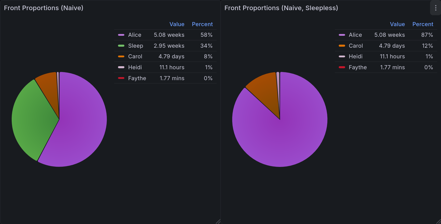
This pair of pie charts shows relative front time when computed naively. Each headmate gets a specific color, keeping things consistent. In the upper right corner of each is a legend showing the color, name, value, and percentage for each of them. The one on the left includes sleep, and the one on the right does not.

Front Time - Combination Aware

A better version of the above would be able to account for those combinations. In this one, our display is modified to list each combination separately, using a canonical ordering to prevent ambiguity. This lets you get much more useful data about system dynamics. For one example, it may be that Carly and Darryl almost always front together.

We can do this by incorporating the concepts we established in the Current Fronters chart. The first two portions are entirely identical, applying the same logic at each step. At the last part, instead of returning a single row we are aggregating the total amount of time for each combination of fronters in the time range.

WITH x AS (
  SELECT start AS chrono FROM joplin.front_tracking
  UNION
  SELECT stop AS chrono FROM joplin.front_tracking
),

y AS (
  SELECT
    x.chrono,
    string_agg(task, ', ' ORDER BY task) AS fronters,
    (lead(chrono) OVER (ORDER BY chrono)) - chrono AS delta
  FROM x LEFT OUTER JOIN joplin.front_tracking
    ON x.chrono >= start AND (x.chrono < stop OR stop IS NULL)
  WHERE chrono IS NOT NULL
  GROUP BY 1 ORDER BY chrono DESC
)

SELECT
  fronters AS "Fronter(s)",
  EXTRACT(EPOCH FROM SUM(CASE
    WHEN delta IS NOT NULL
    THEN delta
    ELSE NOW() - chrono
    END))
FROM y
WHERE (delta IS NULL OR delta > interval '20 seconds')
  AND $__timeFilter(chrono)
GROUP BY "Fronter(s)"

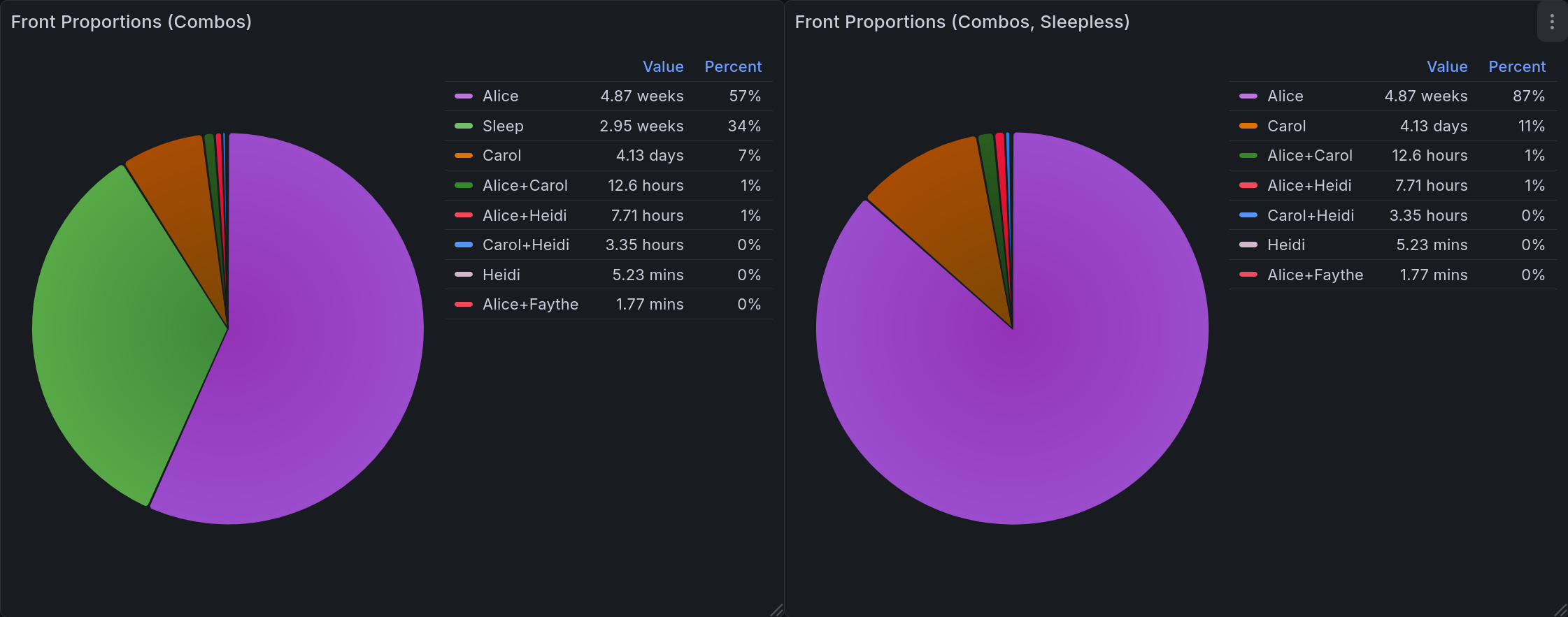
This pair of pie charts shows relative front time when computed with combinations in mind. Groupings are labelled as a + separated string. Each grouping gets a specific color, keeping things consistent. In the upper right corner of each is a legend showing the color, name, value, and percentage for each of them. The one on the left includes sleep, and the one on the right does not.

A Timeline

The other useful view for this data is as a state timeline, as we discussed in the first entry [ACb]. Usefully, the time tracking plugin gives us data in precisely the format we need. The only post-processing we need is to apply the standard partition-by-values filter that we’ve used in most of these other panels.

SELECT
  start AS ts,
  CASE
    WHEN stop IS NULL
    THEN $__timeTo()
    ELSE stop
    END AS stop,
  task
FROM joplin.front_tracking

WHERE $__timeFilter(start) OR $__timeFilter(stop)
ORDER BY
  (task = 'Sleep (Attempt)') DESC,
  sum(duration) OVER (PARTITION BY task) DESC,
  start,
  task

That ORDER BY clause might look a bit odd, so let’s go through it step by step. First, we order by a boolean. This is forcing the sleep tracking to the top, since it’s unlike other entries in the timeline. Next, we order by duration. In the unlikely event there is a tie, we order by the start value and then by the name of the fronter.

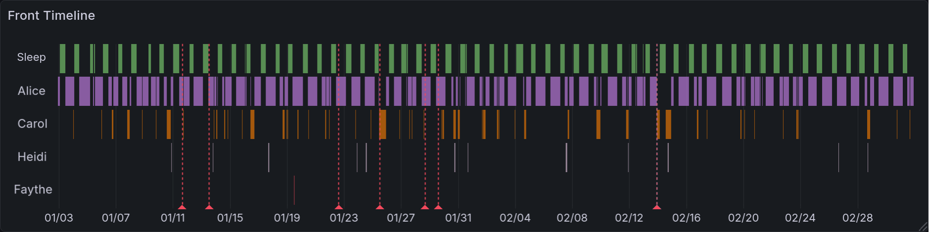
This is the resulting state timeline. Each headmate (and sleeping time) gets a row to mark their times in. When they are fronting, it is highlighted with an assigned color. The headmates are arranged such that the top name fronts the most, and the bottom name the least. Sleep is always at the top. Like several other panels, this has vertical lines that correspond to mental health events (such as arguments, bad news, etc).

Initial Version with Pre-Processing

During the prototyping stage, I was initially looking for combinations while extracting the data from Joplin. This meant that every task, once in the database, would look something like 'Eustace+Franki+Gina'. Any queries that needed individual names would have to parse that out using regular expressions. This was, of course, horribly inefficient. Worse than that, it was brittle and difficult to debug. Being able to do this processing in the query itself is a significant improvement to the developer experience here.

Final Product

I’m quite happy with how I arranged the final dashboards. It was interesting to find an arrangement that kept related information together while not overwhelming. And because (to some extent) this is a demo, I wanted to be sure that I displayed all the interpretations I could reasonably think of. I think I achieved those goals.

System-Specific Dashboard

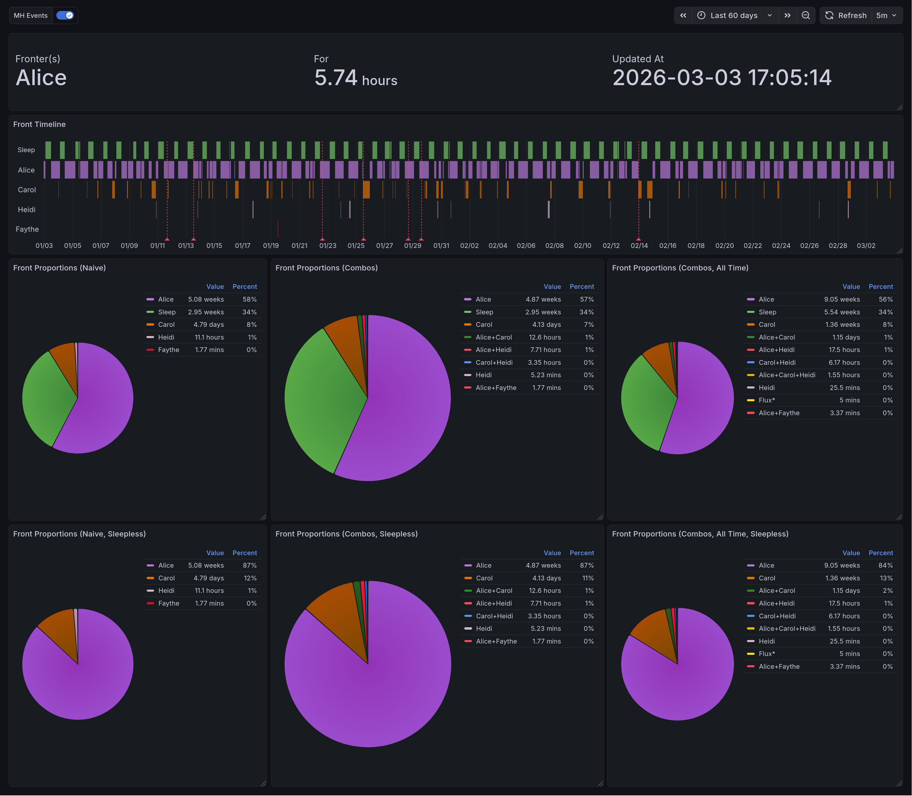
This panel shows the variety of system data we are able to gather. On the top, we have the display of current fronters. Below that is the state timeline which highlights the times when different headmates fronted. Below that is three vertical pairs of pie charts. Each of them is organized such that the version including sleep is on top, and the version excluding sleep is below. On the left are the naively-computed front times. In the middle, and larger than the others, are the combination-aware front times. On the right is a panel displaying combination-aware front time across all historical data.

General Mental Health Dashboard

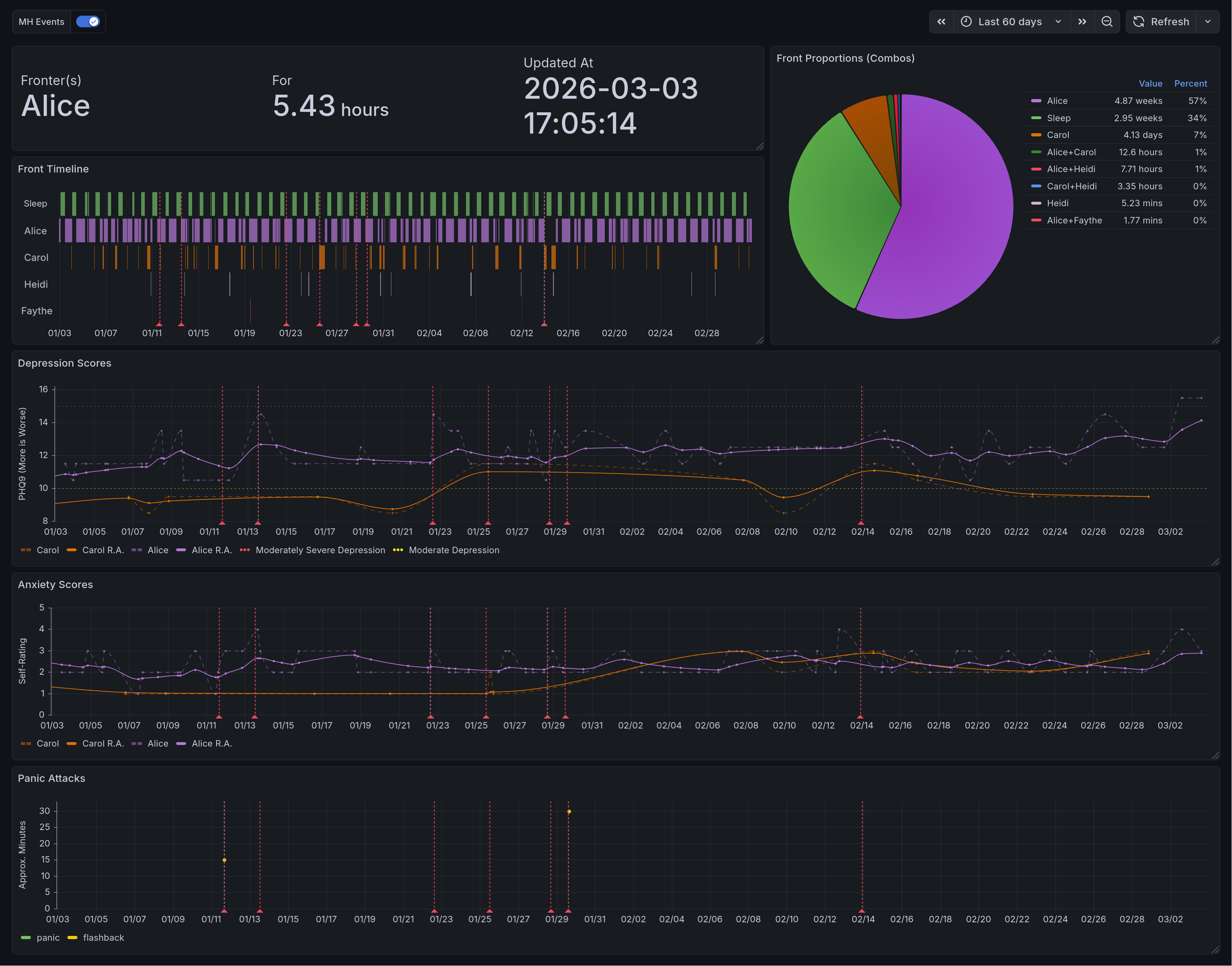
This is the end result for the general dashboard. There are four rows in total. The top row shows system data. The top left of it has the panel of current fronters. Below that is the state timeline of them, and to the right is the combination-aware pie chart. In the second row we have depression scores as computed by the PHQ-9. Below that is self-reported anxiety scores. And lastly you have the panic attack time series.

Main Takeaways

This was a passion project, but it was also a source of many frustrations. I spent a long time working out how to lay out the data, how to phrase questions, how to interpret things. Initially I had it writing this to a spreadsheet and using the built-in charts there, and have slowly been migrating it towards being database-only. Right now it saves to both.

The biggest challenge here was the evolving requirements. Because I was iterating over minimum-viable products, it made it difficult to form a comprehensive design. The benefit, of course, was that I always had something working. I had the motivation of watching it improve, rather than knowing that there were plans that didn’t function yet.

Overall, I would say that I greatly enjoyed working on this. There are many things I would do differently, knowing what I do now, but I am quite proud of what I do have.

Acknowledgments

I greatly appreciate the friends and family who gave feedback for this dashboard along the way. Extra thanks to my friend @Ultralee0@linktr.ee, without whom you would be reading this un-edited. I shudder at the thought. Lastly, I would like to thank the several sensitivity readers who screened this post and offered meaningful suggestions.

Footnotes

[1]

And some horribly-hacky workarounds regarding spreadsheet interactions. Did you know that pyexcel_ods3 has a memory leak at global scope every time you interact with a spreadsheet? Well, I do now, and it means that every time I have to spawn a process just for that purpose or consume infinite memory.

[2] (1,2)

Or for plural folks, who was fronting at the time

[3]

I personally am not a fan of this phrase, I’m just not aware of a better one to use in its stead.

[4]

Not everyone who is plural identifies as a system. Some people find it dehumanizing, prefer other terms, or any myriad of other reasons. I will be using the term in this entry because it seems to be the most common one, but note that it is not the only one.

[5]

This term is sometimes frowned upon because of its origins as a shorthand for “alternate personality” or “alter ego”.

[6]

In this scheme I include “Sleep” as a fronter for ease of processing. That way you can always assume that there is a value for this field.

[7]

It also can exceed 24 hours because the query used here doesn’t know how to slice events to fit perfectly in the sample window. If an event is included, its total time is considered. This is a place for possible improvement.

Citations

[ACa]

Olivia Appleton-Crocker. Lessons in grafana - bonus entry: achieving acceptable averages. URL: https://blog.oliviaappleton.com/posts/0008-lessons-in-grafana-02-5.

[ACb]

Olivia Appleton-Crocker. Lessons in grafana - part one: a vision. URL: https://blog.oliviaappleton.com/posts/0006-lessons-in-grafana-01.

[ACc]

Olivia Appleton-Crocker. Lessons in grafana - part two: litter logs. URL: https://blog.oliviaappleton.com/posts/0007-lessons-in-grafana-02.

[Cur]

National HIV Curriculum. Patient health questionnaire-9 (phq-9). URL: https://www.hiv.uw.edu/page/mental-health-screening/phq-9 (visited on 2026-02-21).

[LFfcad7]

LogarithmicLot and Ffcad7. Separation - pluralpedia. URL: https://pluralpedia.org/index.php?title=Separation&oldid=61671 (visited on 2026-02-08).

[Mit09]

Alex J Mitchell. Why do clinicians have difficulty detecting depression? In Screening for Depression in Clinical Practice: An Evidence-Based Guide. Oxford University Press, 12 2009. URL: https://doi.org/10.1093/oso/9780195380194.003.0006, arXiv:https://academic.oup.com/book/0/chapter/354484514/chapter-pdf/43715552/isbn-9780195380194-book-part-6.pdf, doi:10.1093/oso/9780195380194.003.0006.

[PSTF26]

Nicole Beaulieu Perez, Paula Gordillo Sierra, Brittany Taylor, and Jason Fletcher. Selecting a depression measure for research: a critical examination of five common self-report scales. Journal of Affective Disorders, 394:120542, 2026. URL: https://www.sciencedirect.com/science/article/pii/S0165032725019846, doi:https://doi.org/10.1016/j.jad.2025.120542.

[SSS+]

The Rainy Day System, The Frost System, A Shattered Dragon's Spirit, Pluralanomaly, NeonWebb, Nicolerenee, and LogarithmicLot. Partitionary - pluralpedia. URL: https://pluralpedia.org/index.php?title=Partitionary&oldid=65083 (visited on 2026-02-08).

[Sys]

The Woodland System. Headcount - pluralpedia. URL: https://pluralpedia.org/index.php?title=Headcount&oldid=58294 (visited on 2026-02-08).

Cite As

Click here to expand the bibtex entry.

@online{appleton_blog_0009,
  title    = { Lessons in Grafana - Part Three: Mental Metadata },
  author   = { Olivia Appleton-Crocker },
  editor   = { Ultralee0 },
  language = { English },
  version  = { 1 },
  date     = { 2026-03-09 },
  url      = { https://blog.oliviaappleton.com/posts/0009-lessons-in-grafana-03 }
}

Tags: grafana, data-collection, data-visualization, postgres, postgresQL, python, surveys, mental-health, databases

Comments ,