Achieving Causality with Physical Clocks – A Summary

2025-03-17

During my time at MSU, I had one published paper that mattered to me. It’s a continuation of the HLC paper (my post here). If you haven’t read that, I highly recommend doing so before continuing.

As a review, the Hybrid Logical Clock encodes a form of logical time alongside the physical time information. This allows consumers that are aware of this encoding to enforce causal guarantees. However, it has limitations that are summarized in the table below, which this paper addresses.

Guarantees	Hybrid Logical Clock (HLC)	Physical clocks W/ Causality (PWC)
Very near to NTP time	✅	✅
Uses \(\mathcal{O}(1)\) space	✅	✅
Encodes logical time	✅	✅
Self-stabilizing	✅	✅
Backwards Compatible with NTP	✅	✅
Tolerates large upticks in clock skew	✅	✅
Allows logical time comparision without decoding	❌	✅
Configurable physical precision	❌	✅
On average better physical precision	❌	✅
Tolerates non-monotonic clocks	❌	✅
Tolerates non-constant logical-part size	❌	✅
Allows direct comparison of wall clock time	✅	❌ [1]

The Concept

In the previous paper, they describe a system where the clock maintains three parameters:

• \(l\), a logical clock that’s tied to the physical time

• \(l - pt\), the difference between that and the physical time at the originating node

• \(c\), a counter that acts as a Lamport Clock

This paper simplifies that significantly by eliminating the \(l - pt\) parameter. Doing this allows us to dedicate significantly more memory to the counter portion while also having more precision in the \(l\) parameter. In addition, this lets \(l\) be significantly closer to the physical time. Note that in this new model there are different names assigned to these parameters.

From here on, \(pwc\) shall refer to the entire encoded timestamp. \(clpt\) shall refer to the timestamp where the least-significant \(u\) bits are masked to 0. Under this framing, \(lpt = pwc - clpt\) is analagous to \(c\) in the above description. When we were writing it, I pronounced that as “clean point” and “el point,” though this terminology was not officially adopted. Additionally we have \(hpt = \left\lfloor\tfrac{pwc}{2^u}\right\rfloor\) (pronounced “high point”).

So to review, we have a structure of either 64 (NTP) or 128 bits (NTPv4) that is arranged as:

|------------- pwc ------------|
+------------------------------+
| hpt               | lpt      |
+-------------------+----------+
                    |- u bits -|

The Algorithm

The algorithm at the heart of this looks very similar to that of the previous paper, except with less burden on encoding. If you are generating a local event or sending a message, then:

def on_send(pwc: int, u: int) -> int:
    mask = pow(2, 64) - pow(2, u)
    clpt = physical_clock() & mask
    return max((clpt, pwc + 1))

And on receipt of a message:

def on_receive(pwc: int, m_pwc: int, u: int) -> int:
    mask = pow(2, 64) - pow(2, u)
    clpt = physical_clock() & mask
    return max((clpt, pwc + 1, m_pwc + 1))

Note just how much simpler this is! The whole thing can be boiled down to a couple of conditionals, bitwise operations, and an addition. In fact, it would be trivial to write this in assembly. Clang is able to boil it down to a mere 36 instructions (including 1 function call to get the NTP time). By comparison, the HLC receipt algorithm takes 52 instructions (44% more). It has half the ifs that HLC requires. Plus it has the added benefit that the bit offsets are configurable, unlike in HLC where they are fixed at compile-time.

Determining System Parameters

Now, something you might have been wondering thus far is “how do I determine the value of \(u\)?”

As it turns out, this is going to greatly depend on your expected system layout. Mainly it depends on:

• max expected clock skew (difference between highest and lowest time)

• max expected message delay

• max expected event rate

• max necessary physical time granularity

• network topology

Clock Skew

In essence, clock skew is the amount of disagreement in physical time on the network. This can be because of hardware differences (like if your clock ticks at a slightly different rate) or because of configuration differences (like if your clock ticks correctly, but 10ms in the future). [2]

In practice, we measure clock skew by setting the maximum expected difference between two clocks on a network. You want this to be an overestimate, but as conservative of one as you can manage. So for instance, if the average skew is 1ms, but you know that it can be as high as 10ms 0.1% of the time, you should settle on 10ms.

Message Delay

In this paper, the delay between one node sending a message and the other node receiving it is divided into three parts:

1. \(\delta_{se}\), which is the time it takes to get the message onto the networking device

2. \(\delta_{tr}\), which is the time it takes to get the message to the other node’s networking device

3. \(\delta_{re}\), which is the time it takes for the message to get off the network card and into working memory

Each of these is assumed to be greater than 0, and are a significant factor in determining your value of \(u\).

Time Granularity

The trade-off that you make when you increase \(u\) is that you are reducing the physical-time granularity of your service. If you absolutely need to discern between events separated by 10ns, for instance, you would need to have at \(u \le 5\). Most systems don’t have needs quite that strict, however. Anything that is dealing with ordering human-generated events will likely need at most 0.5ms granularity, which allows for \(u \le 21\).

Final Equation

My proudest work in this paper was on the simulations, so I am going to be somewhat detailed in the findings from that portion. We found that in order to have the maximum time granularity without having wait periods due to the timestamping system, one should set:

\[u \ge \left\lceil \left( \log_2\left( \dfrac{1000 \cdot S^2}{\min(\delta_{re}, \delta_{se})} \right) - \dfrac{\log_2(\epsilon)}{\log_2(S+1)} \right)K^{-1} \right\rceil\]

Where:

• \(K = 2.9 \pm 0.1\) is a weighting constant

• \(S\) is the send rate in messages per node per millisecond

• \(\epsilon\) is the max clock skew in milliseconds

• \(\delta_{re}, \delta_{se}\) are the message receive and message send delays in microseconds

Note that this is significantly better than the naive limit (by about a factor of 3 in most cases), which states:

\[2^u \gt \left\lceil \dfrac{\epsilon}{\min(\delta_{loc},\delta_{re},\delta_{se})} \right\rceil\]

It should also be noted that, while this is not explored thoroughly in the paper, this system can handle a \(u\) parameter that changes over time. There just needs to be a mechanism for coordinating that change. And if some nodes don’t get the memo, you’re still left with the same guarantees as the minimum \(u\) parameter on the network.

Effect of \(\epsilon\), clock skew

In general, we found that every \(K\) doublings of clock skew, you need to add 1 bit to \(u\).

Effect of message rate

An increase of the message rate from a small number (1 / node / ms) to a moderate amount (4 / node / ms) represents a large increase in the needed value of \(u\), but this effect diminishes rather quickly. In general, the higher the message rate, the less important \(\epsilon\) is.

Effect of the number of nodes

We weren’t able to find any real impact from the number of nodes. To quote the paper:

This is predicted by Equation 1 which is independent of the number of nodes. This also makes sense, because a node should expect to see 1 in (N-1) messages from other nodes, and there are (N-1) other nodes sending messages, so these should cancel out as observed.

Effect of network topology

Network topology actually has a large impact not captured by the equations given in this paper. In general, 4 configurations were tested:

1. A random or mesh network, where nodes pick a destination to send to at random

2. A hub-and-spoke network, where nodes send to a central hub that distributes messages

3. A “leader” network, where one clock is arbitrarily ahead of the others, forcing a specific value of \(\epsilon\)

Mesh networks seem to be more resilient to changes in \(\epsilon\). The leader network has a significantly higher baseline value of \(\epsilon\) (as expected) and has a larger variation in minimum-acceptable \(u\) values.

A similar effect is seen in hub-and-spoke networks, likely because large minimum-acceptable \(u\) values propogate more readily. In a mesh network, if one node produces messages with high \(lpt\) values, that will be distributed randomly causing a slow propogation. In a hub-and-spoke network, if the hub node receives such a message it will be distributed very quickly to all other nodes.

In general, this time-keeping schema prefers decentralized networks.

Rare Events

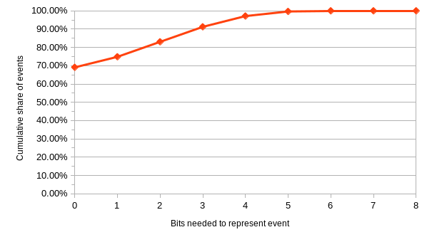
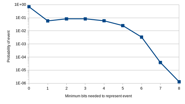
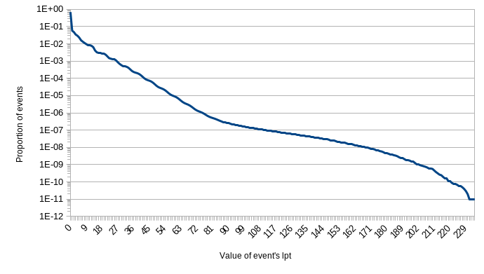
In the paper, I explicitly call out that some simulations showed quite rare events. In particular I point to one with the system parameters: \(\epsilon = 6.25\text{ms}, N=8, S=64\). There were about 736,000,000 events in that run. Of those, about 731,000,000 needed 0 bits allocated to their logical portion. They would be just fine using purely physical time. About 2,000,000 events merely needed 1 bit to distinguish them.

In that simulation we were testing against an expectation of 6 bits being needed. It was able to handle more than that, of course, but we configured it to alert us to any events that would not fit within that space. 27,852 events did not fit, 0.0038% of the total messages.

Only 142 events needed the full 9 bits that we recommend in the abstract. Less than 1 in 1 million.

Below are several charts from the paper detailing these findings.

Conclusions

I personally believe that if you are designing a peer-to-peer protocol, this is the design you should be using for time-keeping. Many of the alternatives are not feasible, either because they require specialized hardware or because they incur too much of a performance cost.

This encoding scheme is incredibly simple and preserves most of the benefits of using a physical clock while integrating the benefits of a logical clock. Importantly, because you can use integer comparisons on the resulting timestamps, it is a drop-in replacement for NTP. Your consumer applications do not need to know the details of this algorithm unless they need more granularity than your networking service offers.

Footnotes

[1]

Skewed by up to \(\epsilon\), where \(\epsilon\) is max expected difference between two clocks on the network + message send delay

[2]

It also can vary based on your gravitational frame, but that’s beyond the scope of this paper. In general, clocks will tick at different rates if you are moving very quickly or experience a different amount of gravity. This is negligible in most network configurations, and is corrected for by NTP.

Citations

Cite As

Click here to expand the bibtex entry.

@online{appleton_blog_0004,
  title    = { Achieving Causality with Physical Clocks — A Summary },
  author   = { Olivia Appleton-Crocker },
  language = { English },
  version  = { 1.1 },
  date     = { 2025-03-17 },
  url      = { https://blog.oliviaappleton.com/posts/0004-PWC }
}

Tags: research-review, msu, published-paper, distributed-systems

Comments ,