Lessons in Grafana - Part Two: Litter Logs

2026-02-23

Welcome back! In this series, I am documenting my journey through data collection and visualization. We’ll be posting one entry a week from now on, until the end of the list below. Today we’re going to be going over my efforts to extract data from our cats’ Litter Robot.

• 1) A Vision

• 2) Litter Logs (you are here)

• 2.5) Achieving Acceptable Averages

• 3) Mental Metadata

• 4) Noticing Notes

• 5) Graphing Goatcounter

• 6) Bridging Gadgets? Biometrics Galore!

• 7) Plotting Prospective Plans

Wait, You’re Getting Data About Cat Bathrooms?

Yes! Isn’t it great?

We initially got this because it significantly reduces the burden of keeping the litterbox clean. It has a number of side benefits, though. There are many different sensors on it, and these get exposed in interesting and semi-processed ways. With the use of the pylitterbot module [SBA+], I have been able to scrape this data.

The biggest benefit of doing so is persistence. Their app shows all of it in a clean way, but they only preserve about 1 month of history. Collecting this data myself means that we can have it indefinitely and without fear of their services losing it. It also means that I get to play around with different things to extract from it!

The Test Subjects

As established by internet law [Bur], I am required to pay the cat tax. Here are our test subjects:

Ophelia (“Loaf”)

Loaf is about 7 years old, and is very people-friendly. If she sees you, she will demand pets. She is the most vocal of our cats by far, and will be very clear if she wants you to follow her. Her favorite hobbies are watching birds and lying between people’s legs.

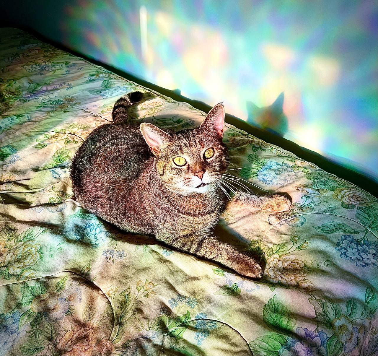
Ophelia, a brown/orange/black cat is laying on a green duvet. Rainbow lights from a nearby window are projected onto the whole image. She is looking up at the camera in curiosity. More pictures can be found on the fedi hashtag #OpheTheLoaf.

Mayalaran (“Maya”)

Maya is about 7 years old, and is quite skittish. She’s gotten a lot more assertive over time, but the starting point was quite low. She is the loudest purrer, and the only one that enjoys belly rubs (in moderation). Her favorite hobbies are judging the neighbors and taking naps.

Maya, a gray cat, is laying in “shrimp pose”, where her front legs are tucked in and her back legs splayed out. Her eyes are half closed, and she is purring very loudly. She is on top of a couch. More pictures can be found on the fedi hashtag #MayalaranTheCat.

Because she is a bit of an anxious princess, Maya doesn’t really use the robot. She did for a little while, but around the time we got Rye she stopped. I think that either the moving parts scare her, or she feels trapped. This means she will not be represented in this data, but I include her anyways since she’s cute.

Pumpernickel (“Rye”)

Rye is about 9 months old, and is a bundle of energy. She has all the tortitude [MRC] and is as distractible as a squirrel after a triple-espresso latte. Her favorite hobbies are wrestling and cuddling.

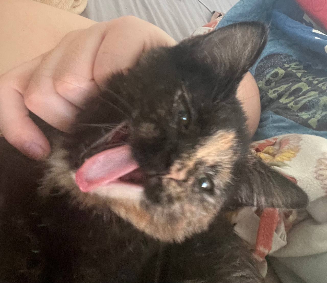
This is Rye as a kitten (roughly 5 months ago). She is a mostly black cat, but with a splash of orange covering most of the right side of her face. She is yawning very wide. More pictures can be found on the fedi hashtag #PumpernickelKitten.

Prerequisites

In the previous entry, I only discussed the Grafana stack itself. We never touched any data collection resources other than entering things by hand. Because of that, there are some things we need to set up. Let’s look at a pared down version of my current data collection workflow, and reason through how it works.

Our first step is to set up database tables. This happens across all of the scrapers I use at the very beginning, and it’s delegated to them to figure things out. In the case of the litterbot scrapers, there are three tables we care about:

Cycle Activity

The simplest table we’ll be collecting is daily cycle activity. The robot has an API endpoint that tells me how many times it ran a cleaning cycle each day. This gives a good general overview of its usage. This data looks like:

CREATE TABLE litterbot.cycle_activity (
   bot_id SMALLINT REFERENCES litterbot.bots(bot_id) ON DELETE CASCADE,
   day DATE NOT NULL,
   cycles SMALLINT NOT NULL,
   PRIMARY KEY (bot_id, day)
)

That’s a lot of jargon, so let’s break it down. The first part is the name of the table itself. This comes in two parts, the first being a schema (in other words, a grouping), and the second being the table name. Grouping things like this allows you to document your work as you go and prevents confusion and any potential conflicts.

The next part tells you each of the columns in the table. The first looks intimidating, but it’s quite simple. You have the ID of a litterbot, and it’s represented by a small number. When that ID is removed from the database, the ON DELETE CASCADE tells you that these entries can also be cleared.

The next items are fairly self-explanatory. They give you the information we’re seeking: a day (in UTC) and how many cleaning cycles were executed.

The last piece does something interesting. It tells the database that you will never have more than one entry for a given bot on a given day. This allows the database to help us sort out any potential conflicts. An example of this might be if you’re fetching the current day. When you look at 6pm, it says there have been 8 cycles. But when you check an hour later, there are 9. This lets us handle those updates automatically in a neat way, and also speeds up searches.

Pet Weights

The most useful table from my perspective is the one that shows our pets’ weights over time. This is especially useful for Rye, as she is supposed to be gaining weight as she grows. It looks like so:

CREATE TABLE litterbot.pet_weight (
   pet_name TEXT NOT NULL,
   ts TIMESTAMP WITH TIME ZONE NOT NULL,
   weight REAL,
   estimated_weight REAL,
   last_weight_reading REAL,
   PRIMARY KEY (pet_name, ts)
)

Here there are some new keywords to look at. First, we have the pet’s name. Next, though, is a timestamp. Above we were giving only a date, since we didn’t need precision. That’s not the case here. Weight measurements are associated with specific times, and the precision of it matters. If you have five entries in a given day, it’s important to distinguish when they happened because you can’t otherwise build a timeline. Suppose the weight suddenly went up. Well, if it’s around dinner time, that’s okay. If not, maybe she got into the cupboard and we should look for missing things. This precision allows for all sorts of storytelling along those lines.

The next three are different versions of the same thing. Because the Litterbot API is odd, it returns three values for the weight. From my perspective, none of these are obvious. They are almost always identical readings, to the point where I suspect this is something that they intended to use, or maybe used on a different product. Functionally you can pretend they are the same thing, and assume we always use the estimated weight value. In this case, note that “real” is used in the math sense. If you think of this as a fraction, that’s close enough.

As before, we set a primary key to help with duplicates. In this case, you’ll never have a pet with two entries at the same time.

This table is by far the most useful to someone like the vet’s office. It gives them weight over time and tells you how frequently they’re going to the bathroom. Those are both valuable insights to have.

Bot Snapshots

The biggest table here is the bot status snapshot. Each time we fetch information, we are able to receive the bot’s status. I record everything that seemed halfway useful. Much of this probably isn’t, but it uses so little space that I may as well.

CREATE TABLE litterbot.bot_snapshot (
   bot_id SMALLINT REFERENCES litterbot.bots(bot_id) ON DELETE CASCADE,
   ts TIMESTAMP WITH TIME ZONE NOT NULL,

   status TEXT,
   power_status TEXT,
   litter_level_state TEXT,
   surface_type TEXT,

   last_seen TIMESTAMP WITH TIME ZONE,
   is_online BOOLEAN,
   is_sleeping BOOLEAN,

   cycle_capacity SMALLINT,
   cycle_count SMALLINT,
   cycles_after_drawer_full SMALLINT,

   litter_level SMALLINT,
   litter_level_calculated SMALLINT,

   waste_drawer_level SMALLINT,
   is_waste_drawer_full BOOLEAN,
   scoops_saved_count INT,

   PRIMARY KEY (bot_id, ts)
)

There’s a number of groupings here. We start with a bot_id and timestamp, as usual. As with the cycle activity, if a bot gets removed from our database, so will all of its corresponding status entries.

The next set is about parsed values. The litterbot API gives a number of indicators for different sensors, and the library I’m using has kindly reverse-engineered the logic of Whisker’s app. The result is four text fields that tell you the most critical issues. status consolidates all of them into a sort of danger signal. power_status tells you what it’s drawing power from (usually “AC”). The litter_level_state tells you whether it’s too full, just right, a bit low, or to “REFILL” right the hell now. Lastly is the surface_type, which I think is set in the app. This tells the bot what type of flooring it’s dealing with, which can affect weight measurements.

The last_seen value was, for a time, the bane of my existence. See, none of this is well-documented. You have to figure out what’s going on for yourself, and I, naively, thought that the last_seen time would update while the device is online. “Oh, we last contacted it ten minutes ago”, things like that. But no. As it turns out, it shows the last time it was offline. If you lose internet at 6pm and gain it back at 6:30pm, that value will stay at 6:30pm until the next time you lose connection. This caused a lot of headaches initially, as I tried to use that as an indicator of when the status was last checked. Unfortunately that doesn’t work, so I use the time of request for that purpose instead. The is_online indicator is tied to that. The is_sleeping indicator is slightly misleading, and seems to indicate the status of an onboard nightlight, rather than indicate that the device is in low power mode.

The cycle grouping is less functional than I would wish for. You would think that cycle_capacity indicated how many cycles could happen before full. That’s not the case. It is instead counting since the last time you emptied the drawer. That’s… less useful, but you could in principle use it to figure out how many cycles go between full states. The next is cycle count, which keeps track of the total number of cleaning cycles the machine has executed. Lastly is cycles_after_drawer_full, which fortunately does exactly what it says. When the robot determines the drawer is full, it will stop cycling. If you force it to do so, it logs that so that it can be upset at you. That value just sits there, silently collecting rage. It doesn’t seem to do anything with it at all.

The litter level grouping is fascinating. Under the hood, what it’s returning is data from a Time of Flight sensor. It is bouncing light[1] off the bottom surface and measuring how long it takes to return. This gives you a fairly precise proxy for how many centimeters of litter you have. Of course, the API doesn’t interpret that data, so that’s left up to pylitterbot. The consequence of this is that the litterbot gives you warnings at 50% empty as measured by time of flight. The calculated value gives a percentage, and the plain one gives raw time of flight.

The last grouping is very similar, but about the waste drawer. It has a percentage level for how full it is, an indicator of if it’s considered full, and a running count of how many scoops it thinks it’s saved you from performing.

These Tables Aren’t Compact. Why?

If you’re a frequent database user, you’ve likely noticed several places in this code where data could be compacted. An example of doing this is with the bot_id field, where it references another table. Why are we not doing that with the pet names? Why are we not doing that with the various status elements?

The reason is relatively simple: it’s not worth it. This portion of the database is very small. At time of writing, it occupies less than 1MiB of total space. I could use all sorts of tricks to reduce that size, but what would be the point? I would need to have about 400 years worth of data before it would occupy 1% of my total disk space. The amount of extra reasoning I would need to do in these queries pales in comparison.

Final Product

Let’s examine the different data displays you can get from this data. All of them have some value, and any time they use tables we didn’t specify above I’ll give a brief summary of what they are.

Litter & Waste Levels

The queries we can use for litter and waste draw levels are delightfully simple, and gives us a good initial case to examine. They look quite similar:

SELECT litter_level_calculated
FROM litterbot.bot_snapshot
ORDER BY ts DESC
LIMIT 1

And

SELECT waste_drawer_level
FROM litterbot.bot_snapshot
ORDER BY ts DESC
LIMIT 1

The first part tells us what values we are looking for. Since each of these queries only read a single value, it’s fairly straightforward. The next bit tells us which table to look in, that we should order it by the time recorded (with most recent first), and that we only want a single entry. This lets us get a very pretty gauge panel, as rendered by [graa]:

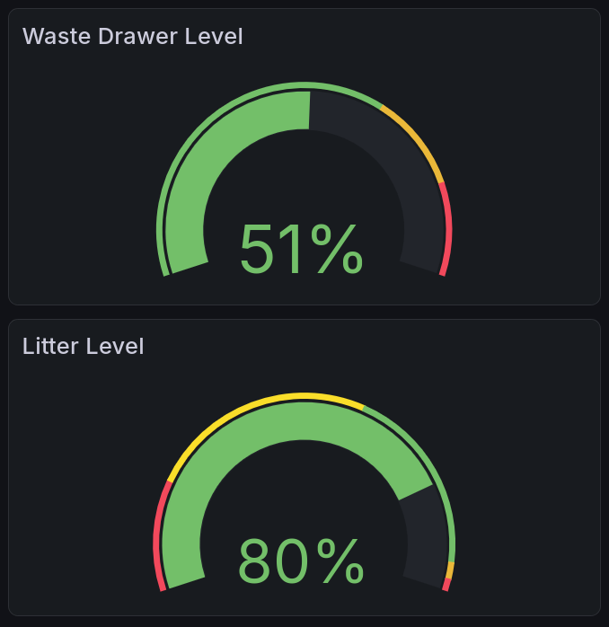
This shows two gauge charts. The top one shows the current level of the waste drawer, and the bottom the current level of the litter reservoir. There is a solid arc of color on each that sweeps to the current level, leaving the rest unfilled.

You’ll notice the gauges have colored sections. We can set these in the configuration for it. In this case, I have tried to reverse-engineer what the app displays, and add some logic for how critical I think it is. For instance, the Whisker app does not distinguish between the fields I label as orange and the fields I label as red.

Current Status

Our current status query is going to look similar to the ones above, except that it is requesting many more values. We’ll look at this in two steps: first with a simplified query, then a hidden section that shows the actual implementation which colors text correctly.

Our query here is as follows:

SELECT
   power_status,
   is_online,
   is_sleeping,
   initcap(status) AS status,
   litter_level_state,
   is_waste_drawer_full
FROM litterbot.bot_snapshot
ORDER BY ts DESC
LIMIT 1

As before, the first part tells us what values we are looking for. This is fairly similar to the above, except for the status field. This is run through a function initcap(), which transforms strings like “aBcDEfG” into “Abcdefg”. This is useful because the status returned by pylitterbot is in all caps, which I find aesthetically displeasing. It will say things like “READY” or “REFILL”, and now in the panel it instead says “Ready” or “Refill”.

Color implementation details here.

Unfortunately this isn’t quite enough to get colors working on the display. Grafana lets you set value mappings for these, but because different columns have different rules for what’s good, we have to distinguish them. I accomplished that by giving prefixes. The resulting query looks like:

SELECT
   power_status,
   CASE
      WHEN is_online THEN 'GYes'
      ELSE 'RNo'
   END AS is_online,
   CASE
      WHEN is_sleeping THEN 'YYes'
      ELSE 'YNo'
   END AS is_sleeping,
   initcap(status) AS status,
   litter_level_state,
   CASE
      WHEN is_waste_drawer_full THEN 'RYes'
      ELSE 'GNo'
   END AS is_waste_drawer_full
from litterbot.bot_snapshot
ORDER BY ts DESC
LIMIT 1

Syntactically this is very similar. What I’ve mainly done is added a letter prefix indicating the color. G indicates it should be green, R that it should be red, and Y that it should be uncolored. Initially I used that for yellow, but it didn’t end up making sense. Then you make a value mapping that removes the prefix and adds the color.

We can render this with Grafana’s Stat plugin [grac], which allows us to render individual values. The result looks like this:

Six status messages are shown side by side. For each of them, there is a smaller title above, with a larger status below. Five of them are colored green, indicating a positive status, and the one labeled “Sleeping?” is colored white because it is status-neutral.

Cycles Per Day

Our cycles per day panel is a time series, as we discussed in the last entry [AC]. You can look there for information on the relevant data format. This panel introduces a new concept for us: time filtering.

SELECT day, cycles
FROM litterbot.cycle_activity
WHERE $__timeFilter(day)

Grafana provides us with a lovely little function, $__timeFilter(), which allows us to look only at data that’s being displayed in the current dashboard. This saves us a lot of effort on data lookup, transfer, and processing. Because we are looking at discrete values rather than one thing changing over time, we use a bar chart to represent it:

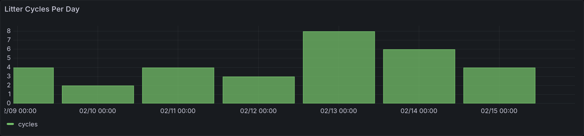
This panel shows a time series rendered with bars. Each bar represents a day’s worth of usage. It is total usage, not partitioned per-cat.

Device Logs

This panel utilizes a table I didn’t describe above, because it’s mostly useful for debugging purposes. The Litterbot produces a log of actions it’s taken, which can be displayed using the Grafana logs plugin [grab]. Our query is as follows:

SELECT ts, action
FROM litterbot.bot_activity
WHERE $__timeFilter(ts)

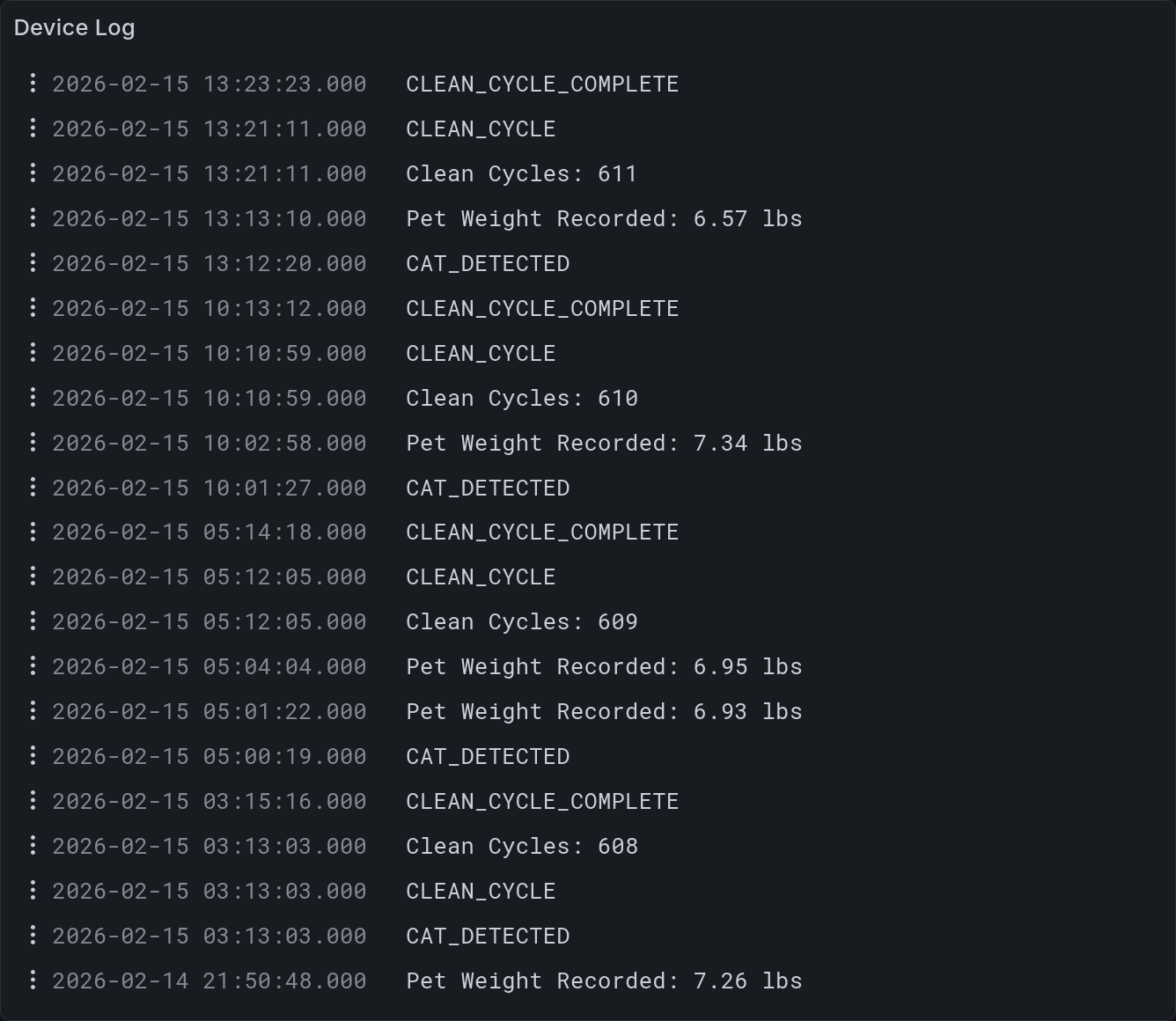
This panel shows the logs generated by the litterbot. They are ordered such that the most recent event is at the top. There is a timestamp on the left for each entry. Some of the entries are raw event statuses, like “CAT_DETECTED”, whereas others are clearly formatted strings, like “Clean Cycles: 611”.

As you can see, this is a fairly useful debug view. You can tell when cats enter, when a cleaning cycle is interrupted, as well as the exact moment it believes that the waste drawer is full. This is more detail than you typically need, but it helps understand what’s going on if presented with suspect data. That’s quite useful.

Per-Pet Usage History

This is, in my opinion, the second most medically-useful chart in this dashboard. It gives you a cumulative view of how often each pet uses the litterbox. Now, this isn’t comprehensive. There is a traditional (read: manually cleaned) litterbox next to it, in part because Maya is an anxious princess and in part so two cats can use the bathroom at once. But this does give a rough proxy, and that is medically useful. It can tell you if they are experiencing digestive issues, or if they’re having trouble urinating, or etc.

An example of this is that Rye recently was sick. She threw up for a while, then had a noticeable uptick in litterbox usage that you can see below. There are alternate explanations for that uptick (for example, she is very easily distractible, and will sometimes go back in because she saw it moving), but this fits very well with the standard progression of a short-term stomach bug. It gives us an indicator that her symptoms are mostly passed.

The query for this is a bit more complex than the others covered here. It uses a UNION statement to combine two data sets. The first part is going to give us a baseline for the time series: everybody starts at 0 times used when the chart begins. The next portion counts how many times a pet appears in the time period we’re looking at.

SELECT DISTINCT
   TIMESTAMP WITH TIME ZONE $__timeFrom() as ts,
   pet_name as pet,
   0 as event
FROM litterbot.pet_weight
UNION ALL
SELECT
   ts,
   pet_name as pet,
   sum(1) OVER (PARTITION BY pet_name ORDER BY ts) as event
FROM litterbot.pet_weight
WHERE $__timeFilter(ts)
ORDER BY pet, ts

Let’s break that down in more detail. The $__timeFrom() function gives us the beginning of the time series chart as set in Grafana. It’s a macro that’s provided to us, and not available in most SQL contexts. We have to specify a type for it because it’s fed in as a raw value. This is much like how we are able to define an interval using a string like '7 days', which you’ll see later in this entry.

In the next SELECT statement you have something new to us: an aggregate function. This is relatively simple. The sum(1) simply counts the number of entries we see. The next bit says what we are counting, which is all values with a matching pet_name ordered by time. This means that for each event we are counting it and all preceding events in the time window.

This query is run through a couple transformations to give us separate datasets. First we tell Grafana to partition the events by the value of pet_name, and then we have a quick rename to remove the prefix that adds to each series. This is a very common pattern in our time series charts, and I will likely not mention it in the future.

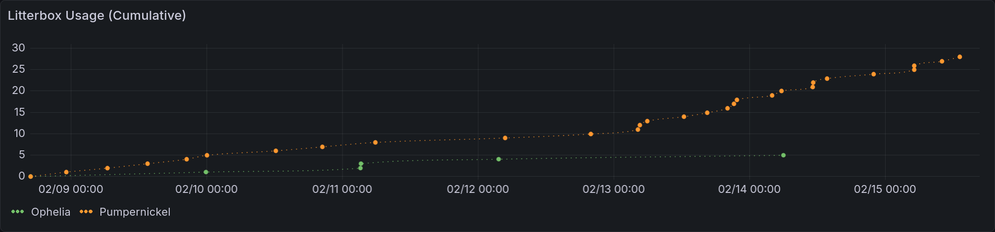
Each cat starts with a point saying 0 usage at the beginning of the time range. From then on, they have a dotted line that connects each additional usage, climbing monotonically. As usual, the orange represents Rye and the green represents Loaf.

Relative Usage Per Pet

This chart is a simplified view of the one above, packed into a pie chart as discussed in the last entry [AC]. It gives relative usage between pets that you can see at a glance. In this case, you can see that Rye used the litterbox about 4 times as often as Loaf did in the last week. This is a bit higher than normal (about 3 times more), probably because she had that stomach bug. I’ll be curious to see if that evens out more as Rye gets older. Kids are usually not good at holding it, after all.

SELECT
   pet_name as pet,
   sum(1) OVER (PARTITION BY pet_name ORDER BY ts) as event
FROM litterbot.pet_weight
WHERE $__timeFilter(ts)
ORDER BY pet

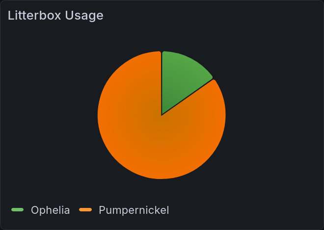
This pie chart reflects overall litterbox usage over the requested period. The orange portion, corresponding to Rye, is much larger than the green portion, corresponding to Loaf.

Per-Pet Weight History

This is the most complicated, and most medically-useful, panel in this dashboard. It gives us pet weights over time, including a running average. That average was really important for me to get right, and it ended up being enough of a project that I detail it in next week’s bonus entry. Stay tuned for that. The query is in five parts:

1. Setting constants

2. Setting up filtering

3. Fetching raw weights

4. Calculating the running average

5. Combining and ordering values

WITH constants AS (
   SELECT interval '4 days' AS half_life
),
-- We're using 4 days as a half-life because it provides a nice smoothing

base AS (
   SELECT *
   FROM constants, litterbot.pet_weight
   WHERE ts < $__timeTo()
      AND ts > (TIMESTAMP WITH TIME ZONE $__timeFrom()) - (half_life * 2)
)
-- This looks like we aren't filtering enough, but that's not true.
-- We want to ensure that our average has enough initial data to work with.

SELECT ts, pet_name AS pet, weight
FROM base
-- This gets the raw weights

UNION ALL

-- and combines it with the running average
SELECT
   ts,
   pet_name || ' R.A.' AS pet,  -- this is string concatenation
   lgbot.ema(
      weight::numeric,
      ts,
      half_life / ln(2)
-- this converts from half-life to expected tau values
   ) OVER (PARTITION BY pet_name ORDER BY ts)
-- and partitioning by pet name means we get that average per-pet
FROM base

ORDER BY pet, ts;
-- And then it gets ordered appropriately

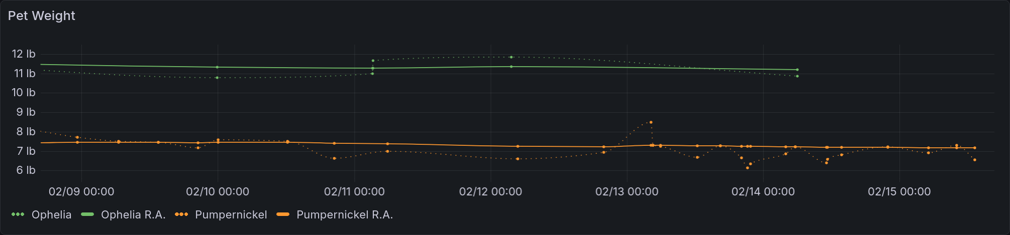
This chart shows a time series of pet weights. There are dotted lines that represent the raw values, and a solid line that represents the time-weighted average. The scale is in US pounds, as that’s what a veterinarian here will want to see (and what the Litterbot exports). Rye has many more weights logged than Loaf, reflecting her greater frequency of usage.

[Insert jokes about not using the metric system here.]

All Together

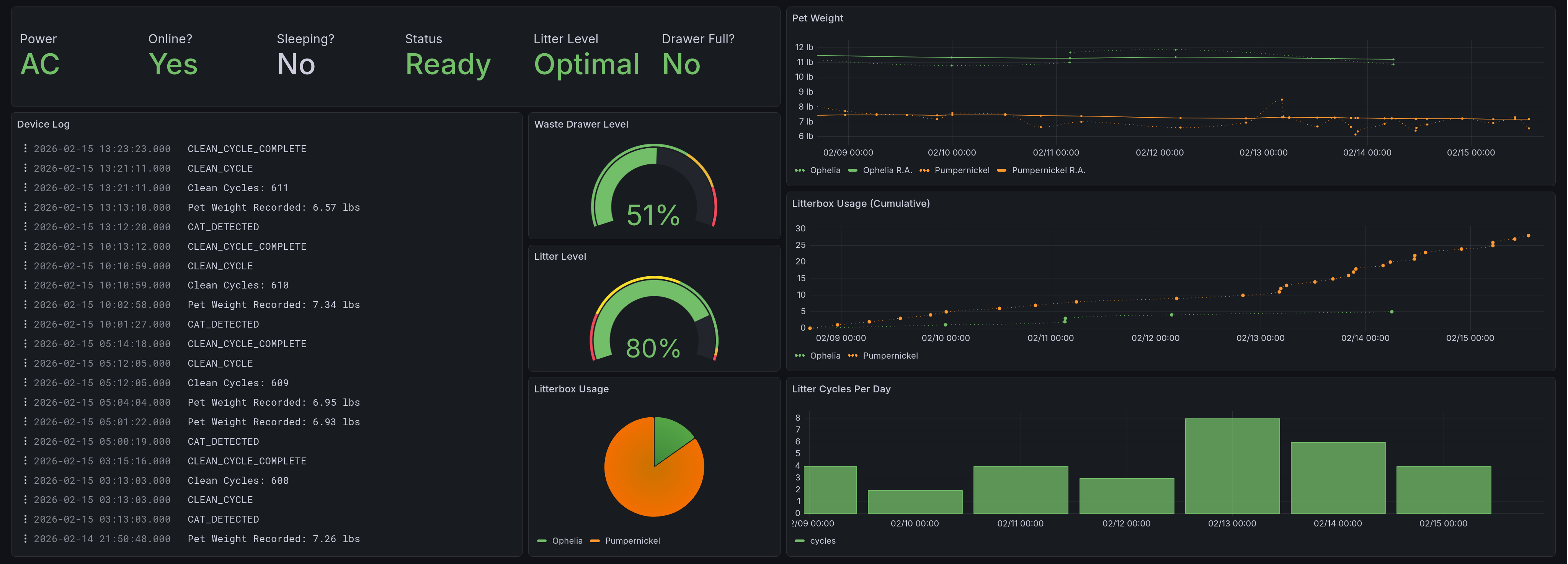
This shows the whole dashboard, giving all of the panels described here. On the top left you see the current status. Below that are two columns, with the one on the left dedicated to the device logs. To the right of that, occupying the middle of the screen, are the gauges and pie chart. From top to bottom we have: waste drawer level, litter level, and relative usage. On the right side of the dashboard we have our three time series. From top to bottom they are: pet weight over time, litterbox usage, and usage per day.

Main Takeaways

I enjoyed making this a lot! When I was writing it, it had the most complicated query I’d implemented in this project. The data collection itself was fairly trivial once I figured out how pylitterbot represented things, and much of the effort went into finding the optimal layout of the database for my purposes. Each of these panels came about because of a specific need, and the data collection I’m performing allows for more to be displayed later on.

The most interesting thing that came out of this was revamping the way I initialize tables. Before this, I had it running CREATE TABLE IF NOT EXISTS for every time it ran. As it turns out, that is terrible for performance. What I do now is create those tables only on startup, and checking that they exist beforehand with a lovely utility function. This was especially useful for the litterbot scraper, as I previously had several indexes and additional tables. The version presented here is much simpler than I initially attempted.

I hope to use this as a model for when I eventually try to collect data from our thermostat and a couple other cat devices.

Next week we dive into the weeds of a specific feature, in a bonus entry: Achieving Acceptable Averages.

Acknowledgments

My gratitude goes to the authors of pylitterbot [SBA+], without whom this work would have been much, much more difficult. Much thanks also goes to my friends @Ultralee0@linktr.ee and Ruby for their thorough test reading of this series.

Footnotes

[1]

Or sound, I suppose. I wasn’t able to find that documented anywhere, but both would work. If it’s sound, then that would be high frequency, which might bother cats. Therefore I assume it’s light.

Citations

[graa]

Grafana gauge visualization. URL: https://grafana.com/docs/grafana/latest/visualizations/panels-visualizations/visualizations/guage/.

[grab]

Grafana logs visualization. URL: https://grafana.com/docs/grafana/latest/visualizations/panels-visualizations/visualizations/logs/ (visited on 2026-02-23).

[grac]

Grafana stat visualization. URL: https://grafana.com/docs/grafana/latest/visualizations/panels-visualizations/visualizations/stat/ (visited on 2026-02-23).

[AC] (1,2)

Olivia Appleton-Crocker. Lessons in grafana - part one: a vision. URL: https://blog.oliviaappleton.com/posts/0006-lessons-in-grafana-01.

[Bur]

Cat Tax Bureau. What is cat tax? meaning, origin & how to pay. URL: https://cat-tax.net/what-is-cat-tax.html (visited on 2026-02-08).

[MRC]

Dr. Lizzie Youens BSc (Hons) BVSc MRCVS. Tortitude: definition, behavior & how to deal with it. URL: https://cats.com/tortitude (visited on 2026-02-15).

[SBA+] (1,2)

Nathan Spencer, Justin Bull, Ian Atha, @jrhe@github.com, Joost Lekkerkerker, Marc Mueller, Ville Skyttä, and Andreas Billmeier. Pylitterbot. Development ongoing. URL: https://github.com/natekspencer/pylitterbot (visited on 2026-02-05).

Cite As

Click here to expand the bibtex entry.

@online{appleton_blog_0007,
  title    = { Lessons in Grafana - Part Two: Litter Logs },
  author   = { Olivia Appleton-Crocker },
  editor   = { Ultralee0 and Ruby },
  language = { English },
  version  = { 1 },
  date     = { 2026-02-23 },
  url      = { https://blog.oliviaappleton.com/posts/0007-lessons-in-grafana-02 }
}

Tags: grafana, data-collection, data-visualization, postgres, postgresQL, python, scraping, databases

Comments ,